Linear Regression
- Will run this together
- ~30 Minutes
- Followed By: A Break!

Learning Objectives
- Define Linear Regression
- Introduce Anscombe's Quartet
- Descriptive Stats of Anscombe's Quartet
- How to test for correlation
- Scatter Plots
- Linear Regression (OLS)
- Visualizing Linear Regression
- QQ Plots
- Prediction with Linear Regression
- Experiment on your own
. . . We have much to discuss.
Linear Regression
Many Data Sets
- R comes with several classic data sets
- R packages come with one or more example data sets
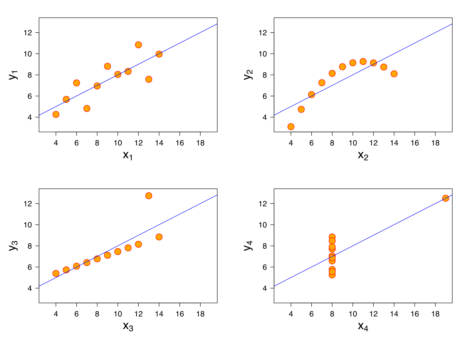
- This presentation relies on Anscombe's Quartet
data()Anscombe's Quartet:
- A (short) break from boat jokes
- First introduced in 1973, used to teach regression
- Four data sets with (nearly) identical statistical properties
- Not identical when plotted!

Anscombe's Quartet (Wikipedia):
Load Data
Anscombe's Quartet is built into R
data(anscombe)
anscombe
  x1 x2 x3 x4    y1   y2    y3    y4
1  10 10 10  8  8.04 9.14  7.46  6.58
2   8  8  8  8  6.95 8.14  6.77  5.76
3  13 13 13  8  7.58 8.74 12.74  7.71
4   9  9  9  8  8.81 8.77  7.11  8.84
5  11 11 11  8  8.33 9.26  7.81  8.47
6  14 14 14  8  9.96 8.10  8.84  7.04
7   6  6  6  8  7.24 6.13  6.08  5.25
8   4  4  4 19  4.26 3.10  5.39 12.50
9  12 12 12  8 10.84 9.13  8.15  5.56
10  7  7  7  8  4.82 7.26  6.42  7.91
11  5  5  5  8  5.68 4.74  5.73  6.89
Many Ways To View An Object
attributes(anscombe)summary(anscombe)str(anscombe)View(anscombe)head(anscombe)tail(anscombe)- R is an object oriented system
- Functions adapt to the object type
Four Distinct Data Sets
| Independent Variable |
Dependent Variable |
|
|---|---|---|
| Set 1 | x1 | y1 |
| Set 2 | x2 | y2 |
| Set 3 | x3 | y3 |
| Set 4 | x4 | y4 |
How Do We Access A Single Column Of Data?
Anscombe's Quartet is a synthetic data set. The abstract ideas which underlie the normal differences between row and column in a data frame do not really apply here. There is relationship between X1 and X3. But, to use the data, we need to access individual columns of data.
Question How can we access all the values in a given colum?
Descriptive Statistics
- It is easy to get the average for each column
- Note: The x columns are nearly identical
- Note: The y columns are nearly identical
colMeans(anscombe)
      x1       x2       x3       x4       y1       y2       y3       y4
9.000000 9.000000 9.000000 9.000000 7.500909 7.500909 7.500000 7.500909
Descriptive Statistics
- Slightly harder to get the standard deviation.
- Note: These are also (essentially) identical
cbind(x1 = sd(anscombe$x1),
      x2 = sd(anscombe$x2),
      x3 = sd(anscombe$x3),
      x4 = sd(anscombe$x4)
      )
          x1       x2       x3       x4
[1,] 3.316625 3.316625 3.316625 3.316625
 Your Turn!
- Can you calculate the standard deviation for the y columns?
Correlation: Set 1
- To test for correlation, we must use an x and y from a single set
cor.test(x=anscombe$x1, y=anscombe$y1)
	Pearson's product-moment correlation

data:  anscombe$x1 and anscombe$y1
t = 4.2415, df = 9, p-value = 0.00217
alternative hypothesis: true correlation is not equal to 0
95 percent confidence interval:
 0.4243912 0.9506933
sample estimates:
      cor
0.8164205
Scatterplot: Set 1
plot(anscombe$x1, anscombe$y1, main="Anscombe: Set 1",
     xlab="x1", ylab="y1"
)

Your Turn!
- Are the correlations of Sets 2 - 4 the same?
- What can you learn from:
?cor.test - Can you reproduce the other scatterplots from Wikipedia?
Linear Regression
m1 <- lm(formula=y1~x1, data=anscombe)
m1
Call:
lm(formula = y1 ~ x1, data = anscombe)

Coefficients:
(Intercept)  anscombe$x1
     3.0001       0.5001
-
To learn more about the R formula syntax for multiple
regression:
?formula
Many Ways To View An Object
attributes(m1)summary(m1)str(m1)View(m1)head(m1)tail(m1)- R is an object oriented system
- Functions adapt to the object type
Many Ways To View An Object
- How much detail do you need?
- Compare results to correlation
summary(m1)
Call:
lm(formula = y1 ~ x1, data = anscombe)

Residuals:
     Min       1Q   Median       3Q      Max
-1.92127 -0.45577 -0.04136  0.70941  1.83882

Coefficients:
            Estimate Std. Error t value Pr(>|t|)
(Intercept)   3.0001     1.1247   2.667  0.02573 *
anscombe$x1   0.5001     0.1179   4.241  0.00217 **
---
Signif. codes:  0 ‘***’ 0.001 ‘**’ 0.01 ‘*’ 0.05 ‘.’ 0.1 ‘ ’ 1

Residual standard error: 1.237 on 9 degrees of freedom
Multiple R-squared:  0.6665,	Adjusted R-squared:  0.6295
F-statistic: 17.99 on 1 and 9 DF,  p-value: 0.00217
Many Ways To Use Objects
- You can access any part of it!
attributes(m1)
$names
 [1] "coefficients"  "residuals"     "effects"       "rank"
 [5] "fitted.values" "assign"        "qr"            "df.residual"
 [9] "xlevels"       "call"          "terms"         "model"

$class
[1] "lm"
attributes(summary(m1))
$names
 [1] "coefficients"  "residuals"     "effects"       "rank"
 [5] "fitted.values" "assign"        "qr"            "df.residual"
 [9] "xlevels"       "call"          "terms"         "model"

$class
[1] "lm"
Many Ways To Use Objects
- How much detail do you want?
m1$coefficients
(Intercept)          x1
3.0000909   0.5000909
summary(m1)$coefficients
             Estimate Std. Error  t value    Pr(>|t|)
(Intercept) 3.0000909  1.1247468 2.667348 0.025734051
anscombe$x1 0.5000909  0.1179055 4.241455 0.002169629
Visualize: Set 1
## Same scatterplot, adds the linear model
plot(anscombe$x1, anscombe$y1, main="Anscombe: Set 1 w/ Model in Red", xlab="x1", ylab="y1")
abline(m1, col="red")

Exporting Graphics
- Exports the Set 1 regression, shown previously
- Exports the file as a PNG file, in the CWD
png("anscombe-1.png")
plot(anscombe$x1, anscombe$y1, main="Anscombe: Set 1 w/ Model in Red", xlab="x1", ylab="y1")
abline(m1, col="red")
dev.off()
Evaluating The Model - QQ PLOT
qqplot(anscombe$x1,anscombe$y1)
abline(m1, col="red")

Your Turn!
- Use a QQ Plot to examine your other models.
- Base R has other tools to evaluate your model:
plot(m1) - Today, our time is limited . . .
Prediction
m1
Call:
lm(formula = y1 ~ x1, data = anscombe)

Coefficients:
(Intercept)           x1
     3.0001       0.5001
Prediction
- Our model is: y = .5001x + 3.0001
- Question: How do we calculate y when x is 10?
-
Answer: We can use R as a calculator!
8.0011 = 10 * .5001 + 3.0001 - But is there an easier way?
Prediction
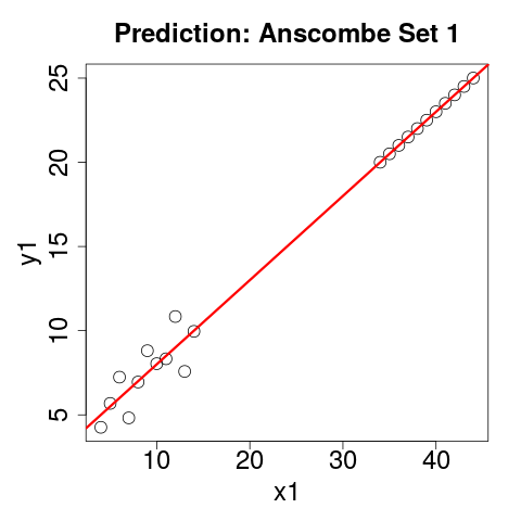
- It is easy to use predict to automate this and do it quickly
- Create a new data.frame with the SAME column names
- The dependent variable must be NA
p1 <- data.frame(x1=anscombe$x1+30, y1=NA)
p1$y1 <- predict(object=m1, newdata=p1)
Let's Look At Our Predictions
plot(rbind(anscombe[,c(1,5)], p1))
abline(m1, col="red")
Prediction Gotcha
- These produce the "same" model
- Only the second can be easily used in a prediction
- Look at the different models produced
- Do you remember how to view the model?
mGood <- lm(formula=y1~x1, data=anscombe)mBad <- lm(formula=anscombe$y1~anscombe$x1)Take A Break!

Titanic in Cobh Harbour, County Cork Ireland